Radar Tutorial

Radar Applications

Radar is a target detection system that uses radio waves to identify the range, altitude, direction, or speed of moving and fixed targets such as aircraft, ships, spacecraft, guided missiles, motor vehicles, weather formations and terrain.The radar dish—or antenna—transmits pulses of radio waves in the microwave range which bounce off any object in their path. The object returns a tiny part of the wave’s energy to the dish or antenna which is usually located at the same site as the transmitter. The information provided by radar includes the bearing and range—and therefore position—of the target. It is thus used in many different fields where the need for such positioning is crucial.

The first use of radar was for military purposes to locate air, ground and sea targets. This has evolved in the civilian field into applications for aircraft, ships and roads.

In aviation, aircraft are equipped with radar devices that warn of obstacles in or approaching their path and give accurate altitude readings. They can land in fog at airports equipped with radar-assisted systems, in which the plane’s flight is observed on radar screens while operators radio landing directions to the pilot.

Marine radars are used to measure the bearing and distance of ships to prevent collision with other ships, to navigate, and to fix their position at sea when within range of shore, or other fixed references such as islands, buoys, and lightships.

Undoubtedly, many of us are intimately familiar with radar guns used by police forces to monitor vehicle speeds on the roads.

Radar has invaded many other fields. Meteorologists use radar to monitor precipitation. It has become the primary tool for short-term weather forecasting and to watch for severe weather such as thunderstorms, tornadoes, and hurricanes. Geologists use specialized ground-penetrating radars to map the composition of the Earth’s crust. The list is getting longer all the time.

Conical Scan Radar

Conical Scan systems send out a signal slightly to one side of the antenna’s boresight and then rotate the feed horn to make the lobe rotate around the boresight line. A target centered on the boresight is always slightly illuminated by the lobe and provides a strong return. If a target is off to one side, it will be illuminated only when the lobe is pointed in that direction which results in a weaker return.

This signal will reach a maximum when the antenna is rotated so that it’s aligned in the direction of the target. By looking for this maximum and moving the antenna in that direction, a target can be tracked automatically. We covered the JPL Deep Space Network in the Fall 1999 issue of the Pentek Pipeline. This network uses rotating radar antennas to support spacecraft missions and radio astronomy observations. The 70-m diameter antenna at Goldstone, CA is shown in Figure 1. Jamming a conical scanning radar is relatively easy. All the jammer has to do is send out signals on the radar’s frequency with enough strength to make it think that it was the strongest return. Jamming of this sort can be made more effective by timing the signals to be the same as the rotational speed of the feed.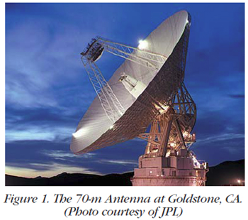

Phased-Array Radar

More recently, in the Spring of 2008 issue, we published a story about a Synthetic Aperture Radar system used by JPL onboard a specially equipped UAV (Unmanned Aerial Vehicle) to study crustal deformation for measuring earthquakes during and after a seismic event. Figure 2 shows the UAV with the radar pod attached to the underside of the aircraft. This phased-array radar utilizes a different method of steering by using either a linear or two-dimensional array of suitablyspaced antenna elements, each with a controllable phase shift. This provides constructive reinforcement of the receive signal or transmit signal for maximum strength in a specific direction. Since phased-array radars require no physical movement, the beam can scan at thousands of degrees per second. Fast enough to track many individual targets and still run a wide-ranging search.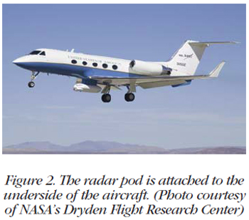

Monopulse Radar

Monopulse radars are similar in general construction to conical scanning systems but with one more feature: instead of sending the signal out of the antenna “as is”, they split it into parts and then send pulsed signals out at slightly different directions. When the reflected signals are received, they are amplified separately and compared to each other; this indicates which direction has the stronger return and therefore the general direction of the target relative to the boresight. Since this comparison is carried out during one pulse, changes in target position or heading have no effect on the comparison.

Making this comparison requires that different parts of the beam be distinguished from each other. This is achieved by splitting the pulse into parts and polarizing each one separately before sending them to a set of slightly off-axis feed horns. This results in a set of lobes overlapping on the boresight. These lobes are rotated as in a normal conical scanner. The two received signals are separated again, one of them is inverted in power to obtain the difference and the two are summed. If the target is to one side of the boresight, the resulting sum will be positive; if it’s on the other, negative.

This system can produce a high degree of accuracy if the lobes are closely spaced. While conical scanning systems generate pointing accuracy on the order of 0.1 degree, monopulse radars improve this by an order of magnitude or better. This amounts to an accuracy of 10 m at a distance of 100 km.

Jamming resistance is also improved over conical scanning systems. Filters can be inserted to remove any signal that’s not polarized or polarized in one direction. In order to confuse such a system, the jamming signal would have to duplicate the polarization and the timing of the monopulse radar.

Monopulse Radar Signal Processing

This is a real-life example of the signal processing involved with a typical monopulse radar application. As shown in Figure 3, the system uses a multi-element antenna where the received signals consist of three types: Azimuth, Elevation and the sum of these two. The signals to be digitized and processed are as follows:

Azimuth difference or ΔA which is equal to A1 – A2 Elevation difference or ΔE which is equal to E1 – E2 Sum Channel Σ which is equal to the sum of A1 + A2 + E1 + E2 The phase shift between Σ and ΔE determines the elevation of the target The phase shift between Σ and ΔA determines the azimuth of the target The IF center frequency of these signals is 140 MHz and the IF bandwidth is 40 MHz This signal processing requires three channels of A/D converters 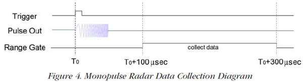Let’s assume that we want to track aircraft targets between a distance of 15 km and 45 km from the radar location. Radar signals travel at the speed of light which is equal to 300,000 km/sec.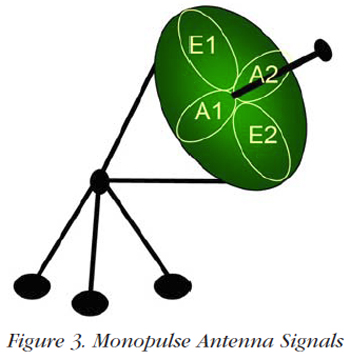

For targets at 15 km, the round trip for the radar pulse takes 2 x 15 km ÷ 300,000 km/sec = 100 μsec. For targets at 45 km, the round trip takes 2 x 45 ÷ 300,000 km/sec = 300 μsec. Figure 4 shows the timing required to collect the data. Generate a 50 μsec pulse at T0; start collecting data at T = T0 + 100 μsec; stop collecting data at T = T0 + 300 μsec.

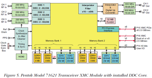
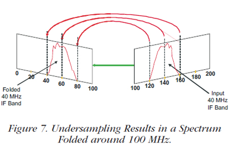
We’ll process the data with the Pentek Cobalt® Model 71621 XMC module shown in Figures 5 and 6. This module is conveniently equipped with three 200 MHz, 16-bit A/Ds. It has a Virtex-6 FPGA, a sample clock synthesizer, a digital upconverter with an interpolator and two 800 MHz, 16-bit D/As, two memory banks as shown in the block diagram, and supports 2.0 GB/sec data transfers over the PCIe interface. To facilitate the signal processing of the monopulse radar system, the 71621 contains three wideband DDC (digital downconverter) cores installed in the Virtex-6 FPGA. These cores provide decimations from 2 to 65,536 and offer independent tuning of the center frequency. To conserve resources, we will try an undersampling solution for digitizing the input signals. If we sample at 200 MHz, the signals of interest will fold as shown in Figure 7: the 120 MHz lower band edge translates to 80 MHz; the 140 MHz center frequency translates to 60 MHz; and the upper band edge translates to 40 MHz. We now need to calculate the decimation setting and the center frequency of the DDC core installed in the 71621: Decimation Setting DEC = 0.8 x ƒs ÷ bandwidth; for a sampling frequency of 200 MHz and a bandwidth of 40 MHz, DEC = 0.8 x 200 ÷ 40 = 4. Our IP core has a range of 2 to 65,536. The undersampling folds the 140 MHz IF to 60 MHz, so the required DDC center frequency tuning is 60 MHz. The IP core tunes from DC to ƒs / 2 or DC to 100 MHz, so the local oscillator is set to 60 MHz. This core handles nicely the required tuning and bandwidth.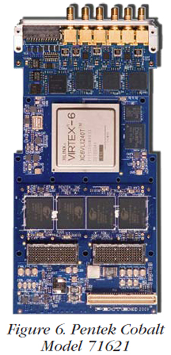

Waveform Signal Generator

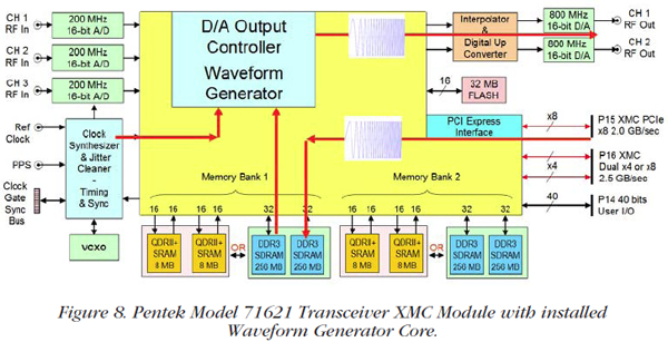
For our next task, we’ll create some radar signals using the Pentek Model 71621 XMC Transceiver module. As shown in Figure 8, the signal waveform is created by the user as a block of digital amplitude samples and loaded across the PCIe interface into the module’s QDR or SDRAM memory. It is then transferred to a waveform engine IP core installed in the Virtex-6 FPGA. The engine delivers the waveform samples to the DUC and the D/As. We can create multiple modes such as triggered, gated, continuous loop, delayed, and so on.

As shown in Figure 9, we chose the complex baseband signal to have 40 MHz bandwidth. When translated to the 140 MHz IF, the 40 MHz signal extends from 120 MHz to 160 MHz. The output sampling frequency must be at least twice the 160 MHz highest frequency, or 320 MHz minimum. Let’s choose 400 MHz to be on the safe side, and use the interpolation filter and DUC to translate the baseband to the IF frequency.

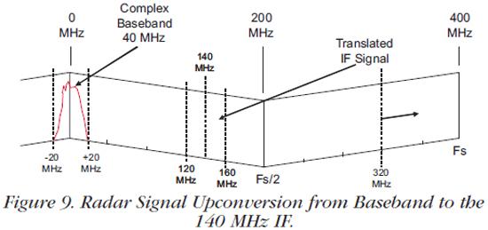
To calculate the interpolation factor for a digital waveform baseband sampling frequency of ƒb; ƒb = 1.25 x Bandwidth, or 1.25 x 40 MHz = 50 MHz. The interpolation factor INT = D/A Output Rate (ƒs) ÷ Baseband Input Rate (ƒb) = 400 MHz ÷ 50 MHz = 8. The interpolation factors available in the DAC5688 are 2, 4 and 8; so we set INT to 8. Range of DUC local oscillator is DC to ƒs / 2 or DC to 200 MHz, so we set the local oscillator to 140 MHz.

Typical parameters for the D/A Output Controller Table are given in Table 1. This table controls the D/A waveform generator and is used to store these parameters in different memory locations. The table entries specify the starting address and waveform length as well as triggering, looping, delays, etc. for the various waveforms to be generated. Each table entry represents a different waveform scenario.

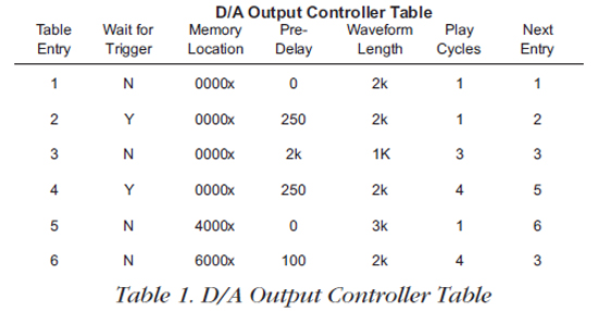
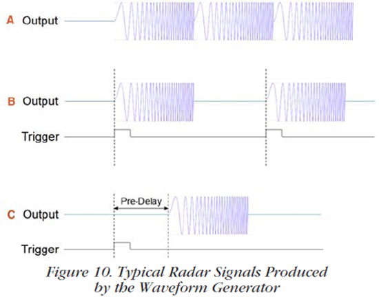
Figure 10 shows three typical waveforms. Waveform A shows a continuous waveform where the generator runs continuously and repeats it in an endless loop. Waveform B is a triggered single and it generates one record for each input trigger. Finally, waveform C is a pre-delay single where the generator waits for a specified delay and then outputs the waveform once.

Radar Pulse Signal Acquisition

To process the received radar data, we will utilize synchronous sampling where we collect A/D samples simultaneously on all three channels. The data collection must be timed precisely to the outgoing trigger pulse. The range gate specifications are precalculated and must be preloaded for fast access.

Just as in the case of the D/A Output Controller Table, the user simply fills in the A/D Input Controller Table such as the one shown in Table 2. The table parameters control the timing of the range gate, specify the memory location for storing the A/D data, the number of samples to store, and the parameters that control triggering, delays, chaining, etc.

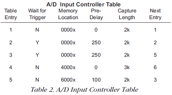
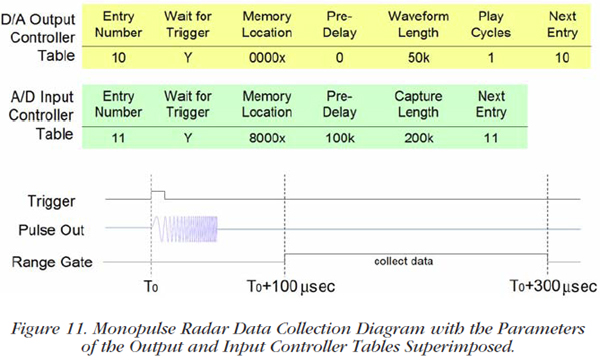
Figure 11 is similar to Figure 4, except here we have superimposed the D/A Output Controller and the A/D Input Controller table entries as they relate to the generation of the outgoing radar pulse and acquisition of the signal returned from the target. The range is the same as given for Figure 4, namely, targets between 15 km and 45 km from the radar location.

Summary

The Pentek Model 71621 Transceiver XMC module is a complete radar signal generation, timing and acquisition subsystem. It has the three A/Ds required for monopulse radar and standard on-board support for signal generation and acquisition timing.

Radar data acquisition is facilitated by the 200 MHz, 16-bit A/Ds which capture the 140 MHz IF signals with 40 MHz bandwidth. Wideband DDC IP cores convert the IF signals down to baseband. The A/D input controller engine uses a simple parameter table that creates programmable delays, acquisition record lengths and complex acquisition scenarios.

Radar waveform generation uses a D/A controller engine with a simple parameter table. It creates multiple waveforms with programmable delays and lengths. The wideband DUC upconverts the digital baseband waveform to 140 MHz IF and the 400 MHz, 16-bit D/A delivers 140 MHz IF signal with 40 MHz bandwidth.